Quickstart

There are two basic ways to use spindler.

• Compute the evolution of a binary system

• Provide the derivatives of the orbital parameters, which can then be used by another package to compute the evolution separately.

import numpy as np
import matplotlib.pyplot as plt

plt.style.use('seaborn-v0_8-darkgrid')
plt.rcParams["mathtext.fontset"]="stix"
plt.rcParams["font.family"]="STIXGeneral"
plt.rcParams["font.size"]=18

Computing the evolution

Compute the evolution of a binary system interacting with a circumbinary disk with the evolve method.

from spindler.solver import Solver_Siwek23, Solver_DD21, Solver_Zrake21

# Define the initial conditions
q0 = 0.7 # initial mass ratio
e0 = 0.1 # initial eccentricity

# Define the mass that will be accreted from the disk
# in units of the initial mass of the binary.
accreted_mass = 0.4 # 40% of the initial mass

# Compute the evolution
a, q, e, m = Solver_Siwek23().evolve(accreted_mass, q0, e0)

fig, ax = plt.subplots()
ax.plot(m,q, label="$q$")
ax.plot(m,e, label="$e$")
ax.plot(m,a, label="$a/a_0$")
ax.set_xlabel("$m/m_0$")
ax.legend()
plt.show()

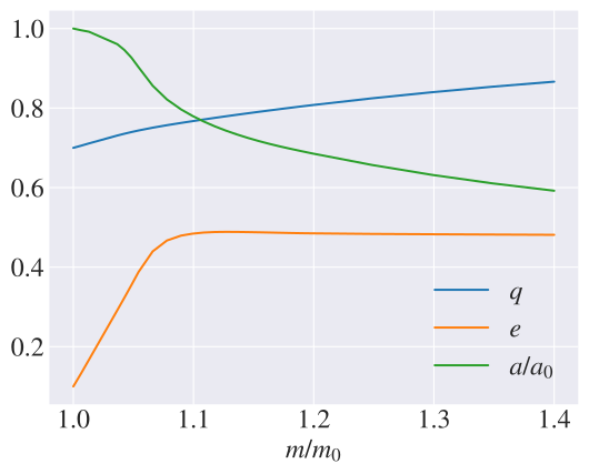
The code would be analogous when using Solver_DD21 or Solver_Zrake21, except that they only support q0=1.

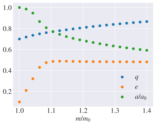
evolve accepts any keyword argument that is accepted by scipy.integrate.solve_ivp. For instance, you can pass the argument t_eval that defines at which values of m you want the solution to be calculated

# Evaluate the solution only at these points
m_eval = np.linspace(1, 1+accreted_mass, 20)
a,q,e,m = Solver_Siwek23().evolve(accreted_mass, q0, e0, t_eval=m_eval)

fig, ax = plt.subplots()
ax.scatter(m,q, label="$q$")
ax.scatter(m,e, label="$e$")
ax.scatter(m,a, label="$a/a_0$")
ax.set_xlabel("$m/m_0$")
ax.legend()
plt.show()

Computing the derivatives of the orbital parameters

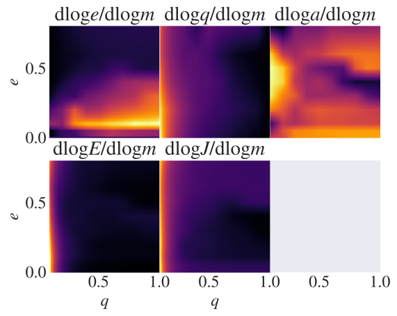
The derivatives are expressed in logaritmic form i.e., the derivative of the quantity \(X\) will be given as

\[\frac{d \log X}{d\log m},\]

where \(m\) is the mass of the binary (the sum of the two components).

Spindler can compute the derivatives of the following quantities: - eccentricity \(e\) - mass ratio \(q\) - semimajor axis \(a\) - orbital energy \(E\) - orbital angular momentum \(J\)

The derivatives can be accessed with the methods get_De, get_Dq, get_De, get_DE, and get_DJ.

solver = Solver_Siwek23()
q_array = np.linspace(0.1,1,100)
e_array = np.linspace(0,0.8,100)
q,e = np.meshgrid(q_array,e_array)

# Compute the derivatives
De = solver.get_De(q,e)
Dq = solver.get_Dq(q,e)
Da = solver.get_Da(q,e)
DE = solver.get_DE(q,e)
DJ = solver.get_DJ(q,e)

fig, axs = plt.subplots(2,3,sharex=True, sharey=True)
fig.subplots_adjust(wspace=0)
cmap = "inferno"
axs[0][0].pcolormesh(q_array,e_array, De, cmap=cmap, rasterized=True)
axs[0][1].pcolormesh(q_array,e_array, Dq, cmap=cmap, rasterized=True)
axs[0][2].pcolormesh(q_array,e_array, Da, cmap=cmap, rasterized=True)
axs[1][0].pcolormesh(q_array,e_array, DE, cmap=cmap, rasterized=True)
axs[1][1].pcolormesh(q_array,e_array, DJ, cmap=cmap, rasterized=True)

axs[0][0].set_title("dlog$e$/dlog$m$")
axs[0][1].set_title("dlog$q$/dlog$m$")
axs[0][2].set_title("dlog$a$/dlog$m$")
axs[1][0].set_title("dlog$E$/dlog$m$")
axs[1][1].set_title("dlog$J$/dlog$m$")
axs[0][0].set_ylabel("$e$")
axs[1][0].set_ylabel("$e$")
axs[1][0].set_xlabel("$q$")
axs[1][1].set_xlabel("$q$")
axs[1][2].grid(False)
plt.show()